前段时间读了 LLM 的书,算是终于了解了 LLM 原理。
不过内容都是偏训练,推理过程介绍较少。趁着假期看了 Fast & Efficient LLM Inference with vLLM 这门课程,时长只有一个半小时,不过加上补课外知识,断断续续花了将近 10 个小时,这里做下一些课堂笔记思考。
课程非常精炼和系统化,对于推理的背景、思路和解决方案都提到了,难得的是还有实战部分,非常推荐。
拿到模型权重文件,最朴素的办法是使用 pytorch 直接加载,然后封装为推理服务。vllm-project 则将这个流程拆分为三段: Optimization → Deploy → Measuring ,分别提出了对应的优化点。
其中 Optimization 有量化和稀疏化,Deploy 有 Continuous Batching, PagedAttention, Prefix Caching 三板斧,这两步的目的都是降低内存和提高计算性能。
Measuring 则是要回答 Cost && Accuracy && Performance 的 tradeoff 问题,有 benchmark(性能指标)、evaluation(业务指标) 两种衡量方式。
接下来展开介绍,首先说下最基础的 KVCache,然后是 Optimization.
1. KVCache
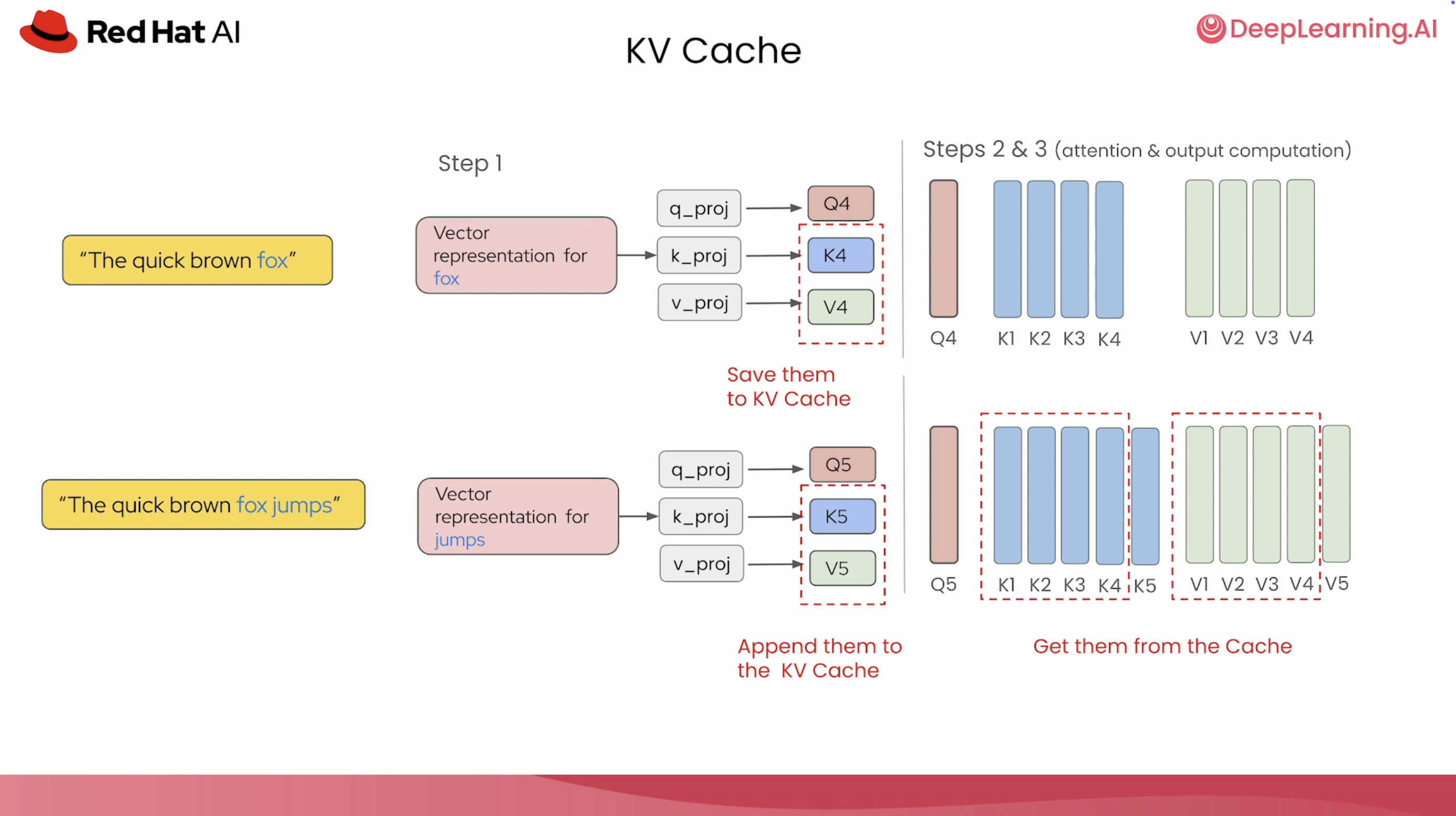
计算 fox 时,我们会得到 K1234 V1234,也就是 The quick brown fox 在 attention 用到的 KV 对。
生成第 5 个 token 时,当前 token 会产生:
\[Q_5,\ K_5,\ V_5\]继续计算 Attention 时,我们还会用到之前的 K1234 V1234. 基于这个观察,为了避免重复计算,自然也就产生了保留上一步 KVCache 的想法。
以上就是最重要的结论。
以下是一些过程说明,不关注可以跳过:
Attention5 的详细计算公式:
\[Attention_5 = softmax \left( \frac{Q_5[K_1,K_2,K_3,K_4,K_5]^T} {\sqrt{d_k}} \right) [V_1,V_2,V_3,V_4,V_5]\]想法很好,但是节省计算同时肯定会导致内存增长,推算的内存公式为:KV * 多少层 * 多头数 * 每头的维度 * 字节数,即
其中:
| 符号 | 含义 |
|---|---|
L |
Transformer Layer 数 |
T |
Token 数 |
H_KV |
KV heads 数 |
D |
head dimension |
bytes |
K/V 数据类型占几个字节 |
2 |
K + V |
例如假定一个 Transformer 有:32 Layer、32 Attention Heads、head_dim = 128
- 每层 Token: 每个 Token 在每一层保存 K V 都需要 32 x 128,加起来就是 2 x 32 x 128 = 8192,如果使用 FP16: 8192 x 2bytes = 16KB
- 32 层:16KB x 32 = 512KB per token
也就是单个 token 的 KVCache 是 512KB,换做 32K tokens: 512KB x 32768 ≈ 16GB 所以这个模型的 32K context,KV Cache 可能已经达到 16GB。更直观的理解: 如果 问题 + 已经生成的答案,总共达到 32K tokens,那么这一条请求本身就可能占掉约 16GB GPU 显存。
2. LLM Compressor-原理
Compressor 的想法跟 GPU 架构强相关:
┌───────────────────────┐
│ GPU SRAM              │ Right next to tensor cores:                            NVIDIA A100:
│ smallest bu fastest   │ specialized hardware for matrix multiplication         20 MB, 19 TB/s
└───────────────────────┘

┌─────────────────────────────────────┐                                          NVIDIA A100:
│ GPU HBM                             │                                          40 GB, 1.5 TB/s
│ smaller than host memory            │
│ but much faster                     │
└───────────────────────▲─────────────┘
                        │ 12GB/s
┌───────────────────────┴───────────────────────────────┐
│ Host Machine's Main Memory                            │
│ CPU DRAM                                              │
│ large but slow                                        │
└───────────────────────────────────────────────────────┘
GPU 可用的内存分为三层:
- GPU SRAM 跟 core 最近,带宽高、内存小;存储计算用到的(极小部分) weights, kvcache, 中间结果
- GPU HBM 稍远,带宽变低,内存变大;存储模型权重、kvcache
- 机器内存,这部分内存最大,带宽也最低;初始化时从磁盘读取一次权重,加载到 HBM 中转使用
tensor cores 计算的数据需要在 SRAM 层读写,因此会不断地从 HBM 搬运到 SRAM, LLM Compressor 的思想,就是能否降低每个参数所需要搬运的字节数(量化),以及让 core 少做无用计算(稀疏化),分别对应了 Quantization 和 Sparsification 两种方法。
- Quantization:量化,比如权重数据用什么格式存储,FP32 → BF16,4 个字节还是 2 字节甚至 1 字节。量化可以作用的范围有模型权重(Weight)、Activations(例如每一层 Transformer 输入、输出的 token 向量表示),所以课程里实际用 W8A16 W8A8 这样描述。量化的直观理解就是降低了对 GPU 的需求,例如 Meta’s Llama 4 有 109B 参数,如果使用 BF16,那就需要 109B * 2bytes ≈ 220GB,大概 3块 80GB 的 GPU,如果能使用 INT4/FP4 存储,就变成了 109B * 0.5 bytes ≈ 55G,使用 1 块 GPU 机器就够了,字节变少,SRAM 从 HBM 一次性读取参数更多,也就是读写更快。
- Sparsification: 稀疏化,把一部分数字变为 0(需要配合计算时跳过这些数字,比如 4 个参数的 tensor,原始
[0.72, -0.13, 0.45, 0.08],稀疏化后[0.72, 0, 0.45, 0], 硬件/算子知道这种结构,然后跳过 0,就从 4 次乘法变成了 2 次乘法),也就是计算更快。
LLM Model 的权重参数是多次训练消耗大量资源生成的,中间也经历了各种设计直到 Transformer 成为主流。然后这里居然可以再次对参数调整,而对推理效果影响很小。这个是我完全没有想到的。最近在读《深度学习入门》这本书,书里提到了这个,起初我还不信。
关于数值精度(用几位数据表示数值),我们已经知道深度学习并不那么需要数值精度的位数。
这块整体上我觉得跟 CPU 的 L1L2L3 Cache 和主存架构类似,思路也让我联想到了brpc 里的 Cacheline
3. LLM Compressor-Code
llm-compressor 是 vLLM 项目出品的生产级量化工具包,封装了上述方法。输入一个已训练好的模型,在一次遍历中降低精度,输出一个体积更小的模型。
核心 API 是 oneshot:传入模型、校准数据集和描述如何量化的 recipe(如 GPTQ, W4A16),产出一个可由 vLLM 直接服务的更小模型。
oneshot(
 model="model-name",           # HuggingFace 模型 ID
 dataset="dataset-name",       # 校准数据集
 recipe=recipe,                # 量化配置
 output_dir="./output",        # 保存位置
 num_calibration_samples=256,  # 校准采样数
 max_seq_length=4096,          # 序列长度
)
recipe 告诉 LLM Compressor 如何量化,是一组 modifier 的列表,每个指定一种算法和设置。
比如我参考课程代码,是这么指定的:
from llmcompressor.modifiers.quantization import GPTQModifier

recipe = GPTQModifier(
    scheme="W4A16",
    targets="Linear",
    ignore=["lm_head"],
)
Modifier即 GPTQ、AWQ 等算法,这里指定即可,课程里也这是简单介绍;scheme 参数决定权重 (W) 和激活 (A) 的位宽,比如 W4A16 表示 Weights 占 4bit,Activations 占 16bit,相比全 FP16 的模型,就是降低了 Weights 参数的精度和大小。targets ignore表示作用于线性层,lm head 仍然保持原来的全精度(embedding默认也是)。
我从 HF 下载Qwen3-0.6B跑了对比:
OUTPUT_DIR = 'Qwen3-0.6B-W4A16-mine'

if not os.path.isdir(OUTPUT_DIR):
    oneshot(
        model="Qwen/Qwen3-0.6B",
        dataset="wikitext",
        dataset_config_name="wikitext-2-raw-v1",
        recipe=recipe,
        output_dir=OUTPUT_DIR,
        max_seq_length=1024, # 课程默认 4096
        num_calibration_samples=32, # 课程默认 256
    )
    print(f"Quantization complete. Model saved to: {OUTPUT_DIR}")
部分核心日志,基本就是在逐层的压缩和计算误差:
  2026-09-26T18:43:48.277491+0800 | from_modifiers | INFO - Creating recipe from modifiers
  2026-09-26T18:43:48.303763+0800 | IndependentPipeline | INFO - Inferred `SequentialPipeline` for `GPTQModifier`
  2026-09-26T18:43:48.309336+0800 | dispatch_for_sequential | WARNING - CUDA/XPU is not available! Compressing model on CPU instead
  2026-09-26T18:44:02.844362+0800 | compress_modules | INFO - Quantizing model.layers.0.self_attn.q_proj using 32 samples
  2026-09-26T18:44:03.267889+0800 | compress | METRIC - error 11.34
  2026-09-26T18:44:03.268465+0800 | compress | METRIC - Compressed module size: 4.243456 MB
  2026-09-26T18:44:03.271242+0800 | compress_modules | INFO - Quantizing model.layers.0.self_attn.k_proj using 32 samples
  2026-09-26T18:56:39.839879+0800 | compress_modules | INFO - Quantizing model.layers.27.mlp.down_proj using 32 samples
  2026-09-26T18:56:40.981504+0800 | compress | METRIC - error 20184.15
  2026-09-26T18:56:51.567524+0800 | finalize | INFO - Compression lifecycle finalized for 1 modifiers
  2026-09-26T18:56:51.573572+0800 | get_model_compressor | INFO - skip_sparsity_compression_stats set to True. Skipping sparsity compression
  statistic calculations. No sparsity compressor will be applied.
  Compressing model: 196it [00:01, 135.74it/s]
  The following generation flags are not valid and may be ignored: ['temperature', 'top_p', 'top_k']. Set `TRANSFORMERS_VERBOSITY=info` for
  more details.
  ✅ 量化完成, 模型保存到: ./models/Qwen3-0.6B-W4A16-mine
模型大小的变化:
Original (BF16):            1.41 GB
Official W4A16 (RedHatAI):  835.3 MB
My W4A16 (GPTQ on target):  528.7 MB
Reduction (mine vs orig):   64%
Reduction (official vs orig):42%
注意:
- 从 16-bit 降到 4-bit(4 倍小),不能预期 75% 的缩减(实际只有 42%)。 原因是只有线性层权重被量化成 Int4,模型的其余部分(包括 LM head 和归一化、Embedding层)保持更高精度。Qwen3 有 15 万词表,所以embedding 参数量 = 151936 × 1024 ≈ 1.56 亿 = 0.156B,占 0.6B 的比例约 25%,也就是 embedding + lm_head 在小模型里占比很高。
- 这里我实际用了三组对比数据,初时的、RedHatAI 优化后的、我自己跑的,因为尝试采用了一些不同的参数,所以虽然都是 W4A16 位宽,但比 RedHatAI 的还要小(当然准确率也下降了),也大概能理解这里其实也是比较吃参数调整和经验的一个活儿。
可以看到 oneshot跑完后体积确实下降了,但是肯定得看效果。如果效果很差,之前的量化工作也没有意义。
主要用两种方式来判断
- 最直接:分别启动模型,看看回答的如何
- 看指标:困惑度,给定数据集,基于前面的文本,模型给出下一步的预测 token 分布,取预期 token 的概率,计算困惑度。也就是模型预测的越精准,困惑度越小。
首先看第一个方式,启动服务:
prompt = "Machine learning is a branch of"

tokenizer = AutoTokenizer.from_pretrained(MODEL_DIR)
base_model = AutoModelForCausalLM.from_pretrained(
    MODEL_DIR, device_map="cpu", dtype=torch.bfloat16,
)

inputs = tokenizer(prompt, return_tensors="pt")
outputs = base_model.generate(
    **inputs,
    max_new_tokens=60,
    do_sample=False,
    pad_token_id=tokenizer.eos_token_id,
)
generated = outputs[0][inputs["input_ids"].shape[-1]:]

print(f"Base Model ({MODEL_DIR})")
print(f"Prompt: {prompt}")
print(f"Response: {tokenizer.decode(generated, skip_special_tokens=True)}")

quant_model = AutoModelForCausalLM.from_pretrained(
    OUTPUT_DIR, device_map="cpu", dtype=torch.bfloat16,
)

inputs = tokenizer(prompt, return_tensors="pt")
outputs = quant_model.generate(
    **inputs,
    max_new_tokens=60,
    do_sample=False,
    pad_token_id=tokenizer.eos_token_id,
)
generated = outputs[0][inputs["input_ids"].shape[-1]:]

print(f"Quantized Model ({OUTPUT_DIR})")
print(f"Prompt: {prompt}")
print(f"Response: {tokenizer.decode(generated, skip_special_tokens=True)}")
从输出看量化后的模型回答的也挺准确:
Base Model (./models/Qwen3-0.6B)
Prompt: Machine learning is a branch of
Response:  artificial intelligence that has gained significant attention in recent years, particularly in the context of the rise of big data and the need for efficient, scalable solutions to complex problems. As the field continues to evolve, the integration of machine learning into various industries is becoming increasingly widespread. However, despite its growing popularity,

Quantized Model (./models/Qwen3-0.6B-W4A16-mine)
Prompt: Machine learning is a branch of
Response:  computer science that uses algorithms to make decisions based on data. It is used to improve the performance of systems and applications by learning from data and making decisions based on that data. It is not a substitute for human intelligence, but it can be used to improve the performance of systems and applications.
然后是困惑度的计算:
def calculate_perplexity(model, tokenizer, dataset, max_tokens=5000, stride=512):
    encodings = tokenizer(
        "\n\n".join(dataset["text"]),
        return_tensors="pt", truncation=True, max_length=max_tokens,
    )
    input_ids = encodings.input_ids
    nlls, prev_end = [], 0

    for begin_loc in range(0, input_ids.size(1), stride):
        end_loc = min(begin_loc + stride, input_ids.size(1))
        trg_len = end_loc - prev_end
        input_slice = input_ids[:, begin_loc:end_loc]
        target_slice = input_slice.clone()
        target_slice[:, :-trg_len] = -100
        with torch.no_grad():
            loss = model(input_slice, labels=target_slice).loss
            nlls.append(loss * trg_len)
        prev_end = end_loc

    return math.exp(torch.stack(nlls).sum() / prev_end)
还是分别用量化前后模型对比:
Base (BF16):      13.37
Quantized (W4A16, Qwen3-0.6B-W4A16-mine): 16.25
Difference:       +2.88 (+21.6%)
指标就能看出来本地跑量化后的模型效果一般,困惑度提高了21.6%,不过这里主要还是参数的问题,课程里的效果比较好(8.2%,我用课程里的 JupyterLab 跑出来是 8.1%)